Data Analysis
Contents
- Data Analysis With Python
Data Analysis With Python
Based on this Cognitive Class Course
Labs
The Labs for the course are located in the Labs folder are from CognitiveClass and are licensed under MIT
Introduction
The data being analysed will be based on a used-car analysis and how to estimate the price of a used car based on its characteristics
- Dataset to be analyzed in Python
- Overview of Python Packages
- Importing and Exporting Data
- Basic Insights from the Data
Understanding the Data
Thhe Data being used is the Autos dataset from the Machine Learning Database at archive.ics.uci
The first few lines of the file are as follows
3,?,alfa-romero,gas,std,two,convertible,rwd,front,88.60,168.80,64.10,48.80,2548,dohc,four,130,mpfi,3.47,2.68,9.00,111,5000,21,27,13495
3,?,alfa-romero,gas,std,two,convertible,rwd,front,88.60,168.80,64.10,48.80,2548,dohc,four,130,mpfi,3.47,2.68,9.00,111,5000,21,27,16500
1,?,alfa-romero,gas,std,two,hatchback,rwd,front,94.50,171.20,65.50,52.40,2823,ohcv,six,152,mpfi,2.68,3.47,9.00,154,5000,19,26,16500
2,164,audi,gas,std,four,sedan,fwd,front,99.80,176.60,66.20,54.30,2337,ohc,four,109,mpfi,3.19,3.40,10.00,102,5500,24,30,13950
2,164,audi,gas,std,four,sedan,4wd,front,99.40,176.60,66.40,54.30,2824,ohc,five,136,mpfi,3.19,3.40,8.00,115,5500,18,22,17450
2,?,audi,gas,std,two,sedan,fwd,front,99.80,177.30,66.30,53.10,2507,ohc,five,136,mpfi,3.19,3.40,8.50,110,5500,19,25,15250
1,158,audi,gas,std,four,sedan,fwd,front,105.80,192.70,71.40,55.70,2844,ohc,five,136,mpfi,3.19,3.40,8.50,110,5500,19,25,17710
1,?,audi,gas,std,four,wagon,fwd,front,105.80,192.70,71.40,55.70,2954,ohc,five,136,mpfi,3.19,3.40,8.50,110,5500,19,25,18920
And the description of the data can be found here, the attributes are as follows
| Column | Attribute | Attribute Range |
|---|---|---|
| 1. | symboling: | -3, -2, -1, 0, 1, 2, 3. |
| 2. | normalized-losses: | continuous from 65 to 256. |
| 3. | make: | alfa-romero, audi, bmw, chevrolet, dodge, honda, isuzu, jaguar, mazda, mercedes-benz, mercury, mitsubishi, nissan, peugot, plymouth, porsche, renault, saab, subaru, toyota, volkswagen, volvo |
| 4. | fuel-type: | diesel, gas. |
| 5. | aspiration: | std, turbo. |
| 6. | num-of-doors: | four, two. |
| 7. | body-style: | hardtop, wagon, sedan, hatchback, convertible. |
| 8. | drive-wheels: | 4wd, fwd, rwd. |
| 9. | engine-location: | front, rear. |
| 10. | wheel-base: | continuous from 86.6 120.9. |
| 11. | length: | continuous from 141.1 to 208.1. |
| 12. | width: | continuous from 60.3 to 72.3. |
| 13. | height: | continuous from 47.8 to 59.8. |
| 14. | curb-weight: | continuous from 1488 to 4066. |
| 15. | engine-type: | dohc, dohcv, l, ohc, ohcf, ohcv, rotor. |
| 16. | num-of-cylinders: | eight, five, four, six, three, twelve, two. |
| 17. | engine-size: | continuous from 61 to 326. |
| 18. | fuel-system: | 1bbl, 2bbl, 4bbl, idi, mfi, mpfi, spdi, spfi. |
| 19. | bore: | continuous from 2.54 to 3.94. |
| 20. | stroke: | continuous from 2.07 to 4.17. |
| 21. | compression-ratio: | continuous from 7 to 23. |
| 22. | horsepower: | continuous from 48 to 288. |
| 23. | peak-rpm: | continuous from 4150 to 6600. |
| 24. | city-mpg: | continuous from 13 to 49. |
| 25. | highway-mpg: | continuous from 16 to 54. |
| 26. | price: | continuous from 5118 to 45400. |
Missing Attribute Values: (denoted by "?")
The Symboling is an indicator of the vehicle risk level, the lower the level the lower the risk (from an insurance level)
The normalized-losses is an indicator of the rate at which the vehicle loses value over time
The price is the value that we would like to predict given the other features
Note that this dataset is from 1995 and therefore the prices may seem a little low
Python Libraries
Scientific Computing Libraries
Pandas
Pandas is a library for working with Data Structures, primarily DataFrames
NumPy
NumPy is a library for working with Arrays and Matrices
SciPy
SciPy includes functions for assisting in mathematical analysis as well as some basic visualizations
Visualization
Matplotlib
Matplotlib is the most commonly used Python library for data visualization
Seaborn
Seaborn is based on Matplotlib and provides functionality such as heat maps, time series, and viollin plots
Algorithmic Libraries
Scikit-learn
Machine learning, regression, classification,etc.
Statsmodels
Explore data, estimate statistical models, and perform statistical tests
Import and Export Data
Importing
When importing data we need ot take a few things into consideration such as
- Format
- File source/path
In our case the data is CSV (.data), and is located as a remote source
We can import our data as follows
import pandas as pd
import numpy as np
# read the online file by the URL provides above, and assign it to variable "df"
path="https://archive.ics.uci.edu/ml/machine-learning-databases/autos/imports-85.data"

df = pd.read_csv(path,header=None)

print("import done")
import done
df.head(2)
| 0 | 1 | 2 | 3 | 4 | 5 | 6 | 7 | 8 | 9 | ... | 16 | 17 | 18 | 19 | 20 | 21 | 22 | 23 | 24 | 25 | |
|---|---|---|---|---|---|---|---|---|---|---|---|---|---|---|---|---|---|---|---|---|---|
| 0 | 3 | ? | alfa-romero | gas | std | two | convertible | rwd | front | 88.6 | ... | 130 | mpfi | 3.47 | 2.68 | 9.0 | 111 | 5000 | 21 | 27 | 13495 |
| 1 | 3 | ? | alfa-romero | gas | std | two | convertible | rwd | front | 88.6 | ... | 130 | mpfi | 3.47 | 2.68 | 9.0 | 111 | 5000 | 21 | 27 | 16500 |
2 rows × 26 columns
We can see that our data comes in without headers, we can assign the headers to our data based on the information in the imports-85.names file
headers = ['symboling','normalized-losses','make','fuel-type','aspiration', 'num-of-doors','body-style',
         'drive-wheels','engine-location','wheel-base', 'length','width','height','curb-weight','engine-type',
         'num-of-cylinders', 'engine-size','fuel-system','bore','stroke','compression-ratio','horsepower',
         'peak-rpm','city-mpg','highway-mpg','price']
df.columns = headers
df.head(10)
| symboling | normalized-losses | make | fuel-type | aspiration | num-of-doors | body-style | drive-wheels | engine-location | wheel-base | ... | engine-size | fuel-system | bore | stroke | compression-ratio | horsepower | peak-rpm | city-mpg | highway-mpg | price | |
|---|---|---|---|---|---|---|---|---|---|---|---|---|---|---|---|---|---|---|---|---|---|
| 0 | 3 | ? | alfa-romero | gas | std | two | convertible | rwd | front | 88.6 | ... | 130 | mpfi | 3.47 | 2.68 | 9.0 | 111 | 5000 | 21 | 27 | 13495 |
| 1 | 3 | ? | alfa-romero | gas | std | two | convertible | rwd | front | 88.6 | ... | 130 | mpfi | 3.47 | 2.68 | 9.0 | 111 | 5000 | 21 | 27 | 16500 |
| 2 | 1 | ? | alfa-romero | gas | std | two | hatchback | rwd | front | 94.5 | ... | 152 | mpfi | 2.68 | 3.47 | 9.0 | 154 | 5000 | 19 | 26 | 16500 |
| 3 | 2 | 164 | audi | gas | std | four | sedan | fwd | front | 99.8 | ... | 109 | mpfi | 3.19 | 3.40 | 10.0 | 102 | 5500 | 24 | 30 | 13950 |
| 4 | 2 | 164 | audi | gas | std | four | sedan | 4wd | front | 99.4 | ... | 136 | mpfi | 3.19 | 3.40 | 8.0 | 115 | 5500 | 18 | 22 | 17450 |
| 5 | 2 | ? | audi | gas | std | two | sedan | fwd | front | 99.8 | ... | 136 | mpfi | 3.19 | 3.40 | 8.5 | 110 | 5500 | 19 | 25 | 15250 |
| 6 | 1 | 158 | audi | gas | std | four | sedan | fwd | front | 105.8 | ... | 136 | mpfi | 3.19 | 3.40 | 8.5 | 110 | 5500 | 19 | 25 | 17710 |
| 7 | 1 | ? | audi | gas | std | four | wagon | fwd | front | 105.8 | ... | 136 | mpfi | 3.19 | 3.40 | 8.5 | 110 | 5500 | 19 | 25 | 18920 |
| 8 | 1 | 158 | audi | gas | turbo | four | sedan | fwd | front | 105.8 | ... | 131 | mpfi | 3.13 | 3.40 | 8.3 | 140 | 5500 | 17 | 20 | 23875 |
| 9 | 0 | ? | audi | gas | turbo | two | hatchback | 4wd | front | 99.5 | ... | 131 | mpfi | 3.13 | 3.40 | 7.0 | 160 | 5500 | 16 | 22 | ? |
10 rows × 26 columns
Next we can remove the missing values from the price column as follows
Analyzing Data
Pandas has a few different methods to undertand the data
We need to do some basic checks such as
- Data Types
- Pandas automatically assigns data types which may not necessarily be correct
- This will further allow us to understand what functions we can apply to what columns
df.dtypes
symboling              int64
normalized-losses     object
make                  object
fuel-type             object
aspiration            object
num-of-doors          object
body-style            object
drive-wheels          object
engine-location       object
wheel-base           float64
length               float64
width                float64
height               float64
curb-weight            int64
engine-type           object
num-of-cylinders      object
engine-size            int64
fuel-system           object
bore                  object
stroke                object
compression-ratio    float64
horsepower            object
peak-rpm              object
city-mpg               int64
highway-mpg            int64
price                 object
dtype: object
We can also view the statisitcal summary as follows
df.describe()
| symboling | wheel-base | length | width | height | curb-weight | engine-size | compression-ratio | city-mpg | highway-mpg | |
|---|---|---|---|---|---|---|---|---|---|---|
| count | 205.000000 | 205.000000 | 205.000000 | 205.000000 | 205.000000 | 205.000000 | 205.000000 | 205.000000 | 205.000000 | 205.000000 |
| mean | 0.834146 | 98.756585 | 174.049268 | 65.907805 | 53.724878 | 2555.565854 | 126.907317 | 10.142537 | 25.219512 | 30.751220 |
| std | 1.245307 | 6.021776 | 12.337289 | 2.145204 | 2.443522 | 520.680204 | 41.642693 | 3.972040 | 6.542142 | 6.886443 |
| min | -2.000000 | 86.600000 | 141.100000 | 60.300000 | 47.800000 | 1488.000000 | 61.000000 | 7.000000 | 13.000000 | 16.000000 |
| 25% | 0.000000 | 94.500000 | 166.300000 | 64.100000 | 52.000000 | 2145.000000 | 97.000000 | 8.600000 | 19.000000 | 25.000000 |
| 50% | 1.000000 | 97.000000 | 173.200000 | 65.500000 | 54.100000 | 2414.000000 | 120.000000 | 9.000000 | 24.000000 | 30.000000 |
| 75% | 2.000000 | 102.400000 | 183.100000 | 66.900000 | 55.500000 | 2935.000000 | 141.000000 | 9.400000 | 30.000000 | 34.000000 |
| max | 3.000000 | 120.900000 | 208.100000 | 72.300000 | 59.800000 | 4066.000000 | 326.000000 | 23.000000 | 49.000000 | 54.000000 |
However, if we want to view a summary including fields that are of type objectm we can do the following
df.describe(include = "all")
| symboling | normalized-losses | make | fuel-type | aspiration | num-of-doors | body-style | drive-wheels | engine-location | wheel-base | ... | engine-size | fuel-system | bore | stroke | compression-ratio | horsepower | peak-rpm | city-mpg | highway-mpg | price | |
|---|---|---|---|---|---|---|---|---|---|---|---|---|---|---|---|---|---|---|---|---|---|
| count | 205.000000 | 205 | 205 | 205 | 205 | 205 | 205 | 205 | 205 | 205.000000 | ... | 205.000000 | 205 | 205 | 205 | 205.000000 | 205 | 205 | 205.000000 | 205.000000 | 205 |
| unique | NaN | 52 | 22 | 2 | 2 | 3 | 5 | 3 | 2 | NaN | ... | NaN | 8 | 39 | 37 | NaN | 60 | 24 | NaN | NaN | 187 |
| top | NaN | ? | toyota | gas | std | four | sedan | fwd | front | NaN | ... | NaN | mpfi | 3.62 | 3.40 | NaN | 68 | 5500 | NaN | NaN | ? |
| freq | NaN | 41 | 32 | 185 | 168 | 114 | 96 | 120 | 202 | NaN | ... | NaN | 94 | 23 | 20 | NaN | 19 | 37 | NaN | NaN | 4 |
| mean | 0.834146 | NaN | NaN | NaN | NaN | NaN | NaN | NaN | NaN | 98.756585 | ... | 126.907317 | NaN | NaN | NaN | 10.142537 | NaN | NaN | 25.219512 | 30.751220 | NaN |
| std | 1.245307 | NaN | NaN | NaN | NaN | NaN | NaN | NaN | NaN | 6.021776 | ... | 41.642693 | NaN | NaN | NaN | 3.972040 | NaN | NaN | 6.542142 | 6.886443 | NaN |
| min | -2.000000 | NaN | NaN | NaN | NaN | NaN | NaN | NaN | NaN | 86.600000 | ... | 61.000000 | NaN | NaN | NaN | 7.000000 | NaN | NaN | 13.000000 | 16.000000 | NaN |
| 25% | 0.000000 | NaN | NaN | NaN | NaN | NaN | NaN | NaN | NaN | 94.500000 | ... | 97.000000 | NaN | NaN | NaN | 8.600000 | NaN | NaN | 19.000000 | 25.000000 | NaN |
| 50% | 1.000000 | NaN | NaN | NaN | NaN | NaN | NaN | NaN | NaN | 97.000000 | ... | 120.000000 | NaN | NaN | NaN | 9.000000 | NaN | NaN | 24.000000 | 30.000000 | NaN |
| 75% | 2.000000 | NaN | NaN | NaN | NaN | NaN | NaN | NaN | NaN | 102.400000 | ... | 141.000000 | NaN | NaN | NaN | 9.400000 | NaN | NaN | 30.000000 | 34.000000 | NaN |
| max | 3.000000 | NaN | NaN | NaN | NaN | NaN | NaN | NaN | NaN | 120.900000 | ... | 326.000000 | NaN | NaN | NaN | 23.000000 | NaN | NaN | 49.000000 | 54.000000 | NaN |
11 rows × 26 columns
We can also use df.info to see the top and bottom thirty rows of the dataframe
If we would like to get a more complete report of the dataset however, we can make use of the pandas_profiling library which will output a full overall data visualisation
import pandas as pd
import pandas_profiling
pd.read_csv('https://raw.githubusercontent.com/mwaskom/seaborn-data/master/planets.csv').profile_report()
Preprocessing Data
Data preprocessing is the process of cleaning the data in order to get data from its raw form to a more usable format
This can include different stages such as
- Missing value handling
- Data formatting
- Data normalization
- Data binning
- Turning categorical values into numerical values
Missing Values
When no data value is stored for a specific feature in an obsevation
Missing data can be represented in many different ways such as ?, N/A, 0 or blank among other ways
In our dataset normalized losses are represented as NaA
We can deal with missing values in a variety of ways
- Check if the correct data can be found
- Drop the feature
- Drop the data entry
- Replace with average or similar datapoints
- Replace with most common value
- Replace based on knowledge about data
- Leave the data as missing data
Dropping missing data can be done with the df.dropna() function, since we have missing values in the price column, which means those rows will need to be dropped
We also need to make use of the inplace=True parameter to modify the actual dataframe
The df.replace() function allows us to replace missing values in the data
df.replace("?", np.nan, inplace = True)
df.head(10)
| symboling | normalized-losses | make | fuel-type | aspiration | num-of-doors | body-style | drive-wheels | engine-location | wheel-base | ... | engine-size | fuel-system | bore | stroke | compression-ratio | horsepower | peak-rpm | city-mpg | highway-mpg | price | |
|---|---|---|---|---|---|---|---|---|---|---|---|---|---|---|---|---|---|---|---|---|---|
| 0 | 3 | NaN | alfa-romero | gas | std | two | convertible | rwd | front | 88.6 | ... | 130 | mpfi | 3.47 | 2.68 | 9.0 | 111 | 5000 | 21 | 27 | 13495 |
| 1 | 3 | NaN | alfa-romero | gas | std | two | convertible | rwd | front | 88.6 | ... | 130 | mpfi | 3.47 | 2.68 | 9.0 | 111 | 5000 | 21 | 27 | 16500 |
| 2 | 1 | NaN | alfa-romero | gas | std | two | hatchback | rwd | front | 94.5 | ... | 152 | mpfi | 2.68 | 3.47 | 9.0 | 154 | 5000 | 19 | 26 | 16500 |
| 3 | 2 | 164 | audi | gas | std | four | sedan | fwd | front | 99.8 | ... | 109 | mpfi | 3.19 | 3.40 | 10.0 | 102 | 5500 | 24 | 30 | 13950 |
| 4 | 2 | 164 | audi | gas | std | four | sedan | 4wd | front | 99.4 | ... | 136 | mpfi | 3.19 | 3.40 | 8.0 | 115 | 5500 | 18 | 22 | 17450 |
| 5 | 2 | NaN | audi | gas | std | two | sedan | fwd | front | 99.8 | ... | 136 | mpfi | 3.19 | 3.40 | 8.5 | 110 | 5500 | 19 | 25 | 15250 |
| 6 | 1 | 158 | audi | gas | std | four | sedan | fwd | front | 105.8 | ... | 136 | mpfi | 3.19 | 3.40 | 8.5 | 110 | 5500 | 19 | 25 | 17710 |
| 7 | 1 | NaN | audi | gas | std | four | wagon | fwd | front | 105.8 | ... | 136 | mpfi | 3.19 | 3.40 | 8.5 | 110 | 5500 | 19 | 25 | 18920 |
| 8 | 1 | 158 | audi | gas | turbo | four | sedan | fwd | front | 105.8 | ... | 131 | mpfi | 3.13 | 3.40 | 8.3 | 140 | 5500 | 17 | 20 | 23875 |
| 9 | 0 | NaN | audi | gas | turbo | two | hatchback | 4wd | front | 99.5 | ... | 131 | mpfi | 3.13 | 3.40 | 7.0 | 160 | 5500 | 16 | 22 | NaN |
10 rows × 26 columns
Next, we can count the missing value in each column
missing_data = df.isnull()
missing_data.head(5)
| symboling | normalized-losses | make | fuel-type | aspiration | num-of-doors | body-style | drive-wheels | engine-location | wheel-base | ... | engine-size | fuel-system | bore | stroke | compression-ratio | horsepower | peak-rpm | city-mpg | highway-mpg | price | |
|---|---|---|---|---|---|---|---|---|---|---|---|---|---|---|---|---|---|---|---|---|---|
| 0 | False | True | False | False | False | False | False | False | False | False | ... | False | False | False | False | False | False | False | False | False | False |
| 1 | False | True | False | False | False | False | False | False | False | False | ... | False | False | False | False | False | False | False | False | False | False |
| 2 | False | True | False | False | False | False | False | False | False | False | ... | False | False | False | False | False | False | False | False | False | False |
| 3 | False | False | False | False | False | False | False | False | False | False | ... | False | False | False | False | False | False | False | False | False | False |
| 4 | False | False | False | False | False | False | False | False | False | False | ... | False | False | False | False | False | False | False | False | False | False |
5 rows × 26 columns
for column in missing_data.columns.values.tolist():
    print(column)
    print (missing_data[column].value_counts())
    print('')
symboling
False    205
Name: symboling, dtype: int64

normalized-losses
False    164
True      41
Name: normalized-losses, dtype: int64

make
False    205
Name: make, dtype: int64

fuel-type
False    205
Name: fuel-type, dtype: int64

aspiration
False    205
Name: aspiration, dtype: int64

num-of-doors
False    203
True       2
Name: num-of-doors, dtype: int64

body-style
False    205
Name: body-style, dtype: int64

drive-wheels
False    205
Name: drive-wheels, dtype: int64

engine-location
False    205
Name: engine-location, dtype: int64

wheel-base
False    205
Name: wheel-base, dtype: int64

length
False    205
Name: length, dtype: int64

width
False    205
Name: width, dtype: int64

height
False    205
Name: height, dtype: int64

curb-weight
False    205
Name: curb-weight, dtype: int64

engine-type
False    205
Name: engine-type, dtype: int64

num-of-cylinders
False    205
Name: num-of-cylinders, dtype: int64

engine-size
False    205
Name: engine-size, dtype: int64

fuel-system
False    205
Name: fuel-system, dtype: int64

bore
False    201
True       4
Name: bore, dtype: int64

stroke
False    201
True       4
Name: stroke, dtype: int64

compression-ratio
False    205
Name: compression-ratio, dtype: int64

horsepower
False    203
True       2
Name: horsepower, dtype: int64

peak-rpm
False    203
True       2
Name: peak-rpm, dtype: int64

city-mpg
False    205
Name: city-mpg, dtype: int64

highway-mpg
False    205
Name: highway-mpg, dtype: int64

price
False    201
True       4
Name: price, dtype: int64
We'll replace the missing data as follows
- Replace by Mean
- "normalized-losses": 41 missing data
- "stroke": 4 missing data
- "bore": 4 missing data
- "horsepower": 2 missing data
- "peak-rpm": 2 missing data
- Replace by Frequency
- "num-of-doors": 2 missing data
- Becase most cars have 4 doors
- "num-of-doors": 2 missing data
- Drop the Roe
- "price": 4 missing data
- Because price is what we want to predict, it does not help if it is not there
- "price": 4 missing data
Normalized Losses
avg_1 = df['normalized-losses'].astype('float').mean(axis = 0)
df['normalized-losses'].replace(np.nan, avg_1, inplace = True)
Bore
avg_2=df['bore'].astype('float').mean(axis=0)
df['bore'].replace(np.nan, avg_2, inplace= True)
Stroke
avg_3 = df["stroke"].astype("float").mean(axis = 0)
df["stroke"].replace(np.nan, avg_3, inplace = True)
Horsepower
avg_4=df['horsepower'].astype('float').mean(axis=0)
df['horsepower'].replace(np.nan, avg_4, inplace= True)
Peak RPM
avg_5=df['peak-rpm'].astype('float').mean(axis=0)
df['peak-rpm'].replace(np.nan, avg_5, inplace= True)
Number of Doors
First we need to check which door count is the most common
df['num-of-doors'].value_counts()
four    114
two      89
Name: num-of-doors, dtype: int64
And then replace invalid values with that
df["num-of-doors"].replace(np.nan, "four", inplace = True)
Price
And then lastly drop the columns with a missing price
df.dropna(subset=["price"], axis=0, inplace = True)

# reset index, because we droped two rows
df.reset_index(drop = True, inplace = True)
Clean Data
The we can view our dataset which has no missing values
df.head()
| symboling | normalized-losses | make | fuel-type | aspiration | num-of-doors | body-style | drive-wheels | engine-location | wheel-base | ... | engine-size | fuel-system | bore | stroke | compression-ratio | horsepower | peak-rpm | city-mpg | highway-mpg | price | |
|---|---|---|---|---|---|---|---|---|---|---|---|---|---|---|---|---|---|---|---|---|---|
| 0 | 3 | 122 | alfa-romero | gas | std | two | convertible | rwd | front | 88.6 | ... | 130 | mpfi | 3.47 | 2.68 | 9.0 | 111 | 5000 | 21 | 27 | 13495 |
| 1 | 3 | 122 | alfa-romero | gas | std | two | convertible | rwd | front | 88.6 | ... | 130 | mpfi | 3.47 | 2.68 | 9.0 | 111 | 5000 | 21 | 27 | 16500 |
| 2 | 1 | 122 | alfa-romero | gas | std | two | hatchback | rwd | front | 94.5 | ... | 152 | mpfi | 2.68 | 3.47 | 9.0 | 154 | 5000 | 19 | 26 | 16500 |
| 3 | 2 | 164 | audi | gas | std | four | sedan | fwd | front | 99.8 | ... | 109 | mpfi | 3.19 | 3.40 | 10.0 | 102 | 5500 | 24 | 30 | 13950 |
| 4 | 2 | 164 | audi | gas | std | four | sedan | 4wd | front | 99.4 | ... | 136 | mpfi | 3.19 | 3.40 | 8.0 | 115 | 5500 | 18 | 22 | 17450 |
5 rows × 26 columns
Formatting Data
Now we nee to ensure that our data is correctly formatted
- Data is usually collected in different places and stored in different formats
- Bringing data into a common standard allows for more meaningful comparison
In order to format data, Pandas comes with some tool for us to use
We can also apply mathematical to our data as well as type conversions and column renames
Sometimes the incorrect data type may be set by default to the correct type, it may be necessary for us to convert our data to the correct type for analysis. We can convert datatypes using the df.astype() function, and check types with df.dtypes
Data Types
df.dtypes
symboling              int64
normalized-losses     object
make                  object
fuel-type             object
aspiration            object
num-of-doors          object
body-style            object
drive-wheels          object
engine-location       object
wheel-base           float64
length               float64
width                float64
height               float64
curb-weight            int64
engine-type           object
num-of-cylinders      object
engine-size            int64
fuel-system           object
bore                  object
stroke                object
compression-ratio    float64
horsepower            object
peak-rpm              object
city-mpg               int64
highway-mpg            int64
price                 object
dtype: object
Convert types
We can easily convert our data to the correct types with
df[['bore', 'stroke']] = df[['bore', 'stroke']].astype('float')
df[['normalized-losses']] = df[['normalized-losses']].astype('int')
df[['price']] = df[['price']].astype('float')
df[['peak-rpm']] = df[['peak-rpm']].astype('float')
And view the corrected types
df.dtypes
symboling              int64
normalized-losses      int64
make                  object
fuel-type             object
aspiration            object
num-of-doors          object
body-style            object
drive-wheels          object
engine-location       object
wheel-base           float64
length               float64
width                float64
height               float64
curb-weight            int64
engine-type           object
num-of-cylinders      object
engine-size            int64
fuel-system           object
bore                 float64
stroke               float64
compression-ratio    float64
horsepower            object
peak-rpm             float64
city-mpg               int64
highway-mpg            int64
price                float64
dtype: object
Standardization
Standardization is the process of taking data from one format to another that may be more meaningful for us to use, such as converting our fuel consumption
# transform mpg to L/100km by mathematical operation (235 divided by mpg)
df['city-L/100km'] = 235/df['city-mpg']
df[['city-mpg','city-L/100km']].head()
| city-mpg | city-L/100km | |
|---|---|---|
| 0 | 21 | 11.190476 |
| 1 | 21 | 11.190476 |
| 2 | 19 | 12.368421 |
| 3 | 24 | 9.791667 |
| 4 | 18 | 13.055556 |
df.head()
| symboling | normalized-losses | make | fuel-type | aspiration | num-of-doors | body-style | drive-wheels | engine-location | wheel-base | ... | fuel-system | bore | stroke | compression-ratio | horsepower | peak-rpm | city-mpg | highway-mpg | price | city-L/100km | |
|---|---|---|---|---|---|---|---|---|---|---|---|---|---|---|---|---|---|---|---|---|---|
| 0 | 3 | 122 | alfa-romero | gas | std | two | convertible | rwd | front | 88.6 | ... | mpfi | 3.47 | 2.68 | 9.0 | 111 | 5000.0 | 21 | 27 | 13495.0 | 11.190476 |
| 1 | 3 | 122 | alfa-romero | gas | std | two | convertible | rwd | front | 88.6 | ... | mpfi | 3.47 | 2.68 | 9.0 | 111 | 5000.0 | 21 | 27 | 16500.0 | 11.190476 |
| 2 | 1 | 122 | alfa-romero | gas | std | two | hatchback | rwd | front | 94.5 | ... | mpfi | 2.68 | 3.47 | 9.0 | 154 | 5000.0 | 19 | 26 | 16500.0 | 12.368421 |
| 3 | 2 | 164 | audi | gas | std | four | sedan | fwd | front | 99.8 | ... | mpfi | 3.19 | 3.40 | 10.0 | 102 | 5500.0 | 24 | 30 | 13950.0 | 9.791667 |
| 4 | 2 | 164 | audi | gas | std | four | sedan | 4wd | front | 99.4 | ... | mpfi | 3.19 | 3.40 | 8.0 | 115 | 5500.0 | 18 | 22 | 17450.0 | 13.055556 |
5 rows × 27 columns
df['highway-L/100km'] = 235/df['highway-mpg']
df[['highway-mpg','highway-L/100km']].head()
| highway-mpg | highway-L/100km | |
|---|---|---|
| 0 | 27 | 8.703704 |
| 1 | 27 | 8.703704 |
| 2 | 26 | 9.038462 |
| 3 | 30 | 7.833333 |
| 4 | 22 | 10.681818 |
df.head()
| symboling | normalized-losses | make | fuel-type | aspiration | num-of-doors | body-style | drive-wheels | engine-location | wheel-base | ... | bore | stroke | compression-ratio | horsepower | peak-rpm | city-mpg | highway-mpg | price | city-L/100km | highway-L/100km | |
|---|---|---|---|---|---|---|---|---|---|---|---|---|---|---|---|---|---|---|---|---|---|
| 0 | 3 | 122 | alfa-romero | gas | std | two | convertible | rwd | front | 88.6 | ... | 3.47 | 2.68 | 9.0 | 111 | 5000.0 | 21 | 27 | 13495.0 | 11.190476 | 8.703704 |
| 1 | 3 | 122 | alfa-romero | gas | std | two | convertible | rwd | front | 88.6 | ... | 3.47 | 2.68 | 9.0 | 111 | 5000.0 | 21 | 27 | 16500.0 | 11.190476 | 8.703704 |
| 2 | 1 | 122 | alfa-romero | gas | std | two | hatchback | rwd | front | 94.5 | ... | 2.68 | 3.47 | 9.0 | 154 | 5000.0 | 19 | 26 | 16500.0 | 12.368421 | 9.038462 |
| 3 | 2 | 164 | audi | gas | std | four | sedan | fwd | front | 99.8 | ... | 3.19 | 3.40 | 10.0 | 102 | 5500.0 | 24 | 30 | 13950.0 | 9.791667 | 7.833333 |
| 4 | 2 | 164 | audi | gas | std | four | sedan | 4wd | front | 99.4 | ... | 3.19 | 3.40 | 8.0 | 115 | 5500.0 | 18 | 22 | 17450.0 | 13.055556 | 10.681818 |
5 rows × 28 columns
Renaming Columns
If there is a need for us to rename columns we can do so with df.rename(), for example
df.rename(columns={'"highway-mpg"':'highway-consumption'}, inplace=True)
Data Normalization
This is an important part of data preprocessing
We may need to normalize our variables such that the range of our data is more consistent, allowing us to manage the way that different values will impact our analysis
There are several differnet ways to normalize data
Simple Feature Scaling
df['length'] = df['length']/df['length'].max()
Min-Max
df['length'] = (df['length']-df['length'].min())/
               (df['length'].max()-df['length'].min())
Z-Score
The resulting values hover around zero, and are in terms of their standard deviation from the mean
df['length'] = (df['length']-df['length'].mean())/
               df['length'].std()
Normalization
Next we will normalize our values using the Simple Feature Scaling Method
We will apply this to the following features
- 'length'
- 'width'
- 'height'
df['length'] = df['length']/df['length'].max()
df['width'] = df['width']/df['width'].max()
df['height'] = df['height']/df['height'].max()
df[["length","width","height"]].head()
| length | width | height | |
|---|---|---|---|
| 0 | 0.811148 | 0.890278 | 0.816054 |
| 1 | 0.811148 | 0.890278 | 0.816054 |
| 2 | 0.822681 | 0.909722 | 0.876254 |
| 3 | 0.848630 | 0.919444 | 0.908027 |
| 4 | 0.848630 | 0.922222 | 0.908027 |
Binning
Binning is grouping values together into bins, this can sometimes improve accuracy of predictive models and help us to better understand the data distribution
We'll arrange our 'horsepower' column into bins such that we can label cars as having a 'Low', 'Medium', or 'High' horsepower as follows
df["horsepower"]=df["horsepower"].astype(float, copy=True)
binwidth = (max(df["horsepower"])-min(df["horsepower"]))/4
bins = np.arange(min(df["horsepower"]), max(df["horsepower"]), binwidth)
bins
array([ 48. , 101.5, 155. , 208.5])
We can then use pd.cut() to determine what bin each value belongs in
group_names = ['Low', 'Medium', 'High']
df['horsepower-binned'] = pd.cut(df['horsepower'], bins, labels=group_names,include_lowest=True )
df[['horsepower','horsepower-binned']].head(20)
| horsepower | horsepower-binned | |
|---|---|---|
| 0 | 111.0 | Medium |
| 1 | 111.0 | Medium |
| 2 | 154.0 | Medium |
| 3 | 102.0 | Medium |
| 4 | 115.0 | Medium |
| 5 | 110.0 | Medium |
| 6 | 110.0 | Medium |
| 7 | 110.0 | Medium |
| 8 | 140.0 | Medium |
| 9 | 101.0 | Low |
| 10 | 101.0 | Low |
| 11 | 121.0 | Medium |
| 12 | 121.0 | Medium |
| 13 | 121.0 | Medium |
| 14 | 182.0 | High |
| 15 | 182.0 | High |
| 16 | 182.0 | High |
| 17 | 48.0 | Low |
| 18 | 70.0 | Low |
| 19 | 70.0 | Low |
Visualization
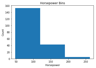
We can use matplotlib to visualize the number of vehicles in each of our bins with the following
%matplotlib inline
from matplotlib import pyplot as plt

a = (0,1,2)

# draw historgram of attribute "horsepower" with bins = 3
plt.hist(df["horsepower"], bins = 3)

# set x/y labels and plot title
plt.xlabel("Horsepower")
plt.ylabel("Count")
plt.title("Horsepower Bins")
plt.show()
Categorical to Quantatative
Most statistical models cannot take in objects as strings, in order to do this we provide a dummy variable that contains whether or not an entry is a certain string variable, we can do this in pandas with pd.get_dummies()
This method will automatically generate a dummy vector for the provided dataframe, and is used as follows
dummy_value = pd.get_dummies(df['value'])
Fuel
We will do this for the 'fuel-type' column in our data
dummy_fuel = pd.get_dummies(df["fuel-type"])
dummy_fuel.head()
| diesel | gas | |
|---|---|---|
| 0 | 0 | 1 |
| 1 | 0 | 1 |
| 2 | 0 | 1 |
| 3 | 0 | 1 |
| 4 | 0 | 1 |
Then we will rename our columns for clarity
dummy_fuel.rename(columns={'gas':'fuel-type-gas', 'diesel':'fuel-type-diesel'}, inplace=True)
dummy_fuel.head()
| fuel-type-diesel | fuel-type-gas | |
|---|---|---|
| 0 | 0 | 1 |
| 1 | 0 | 1 |
| 2 | 0 | 1 |
| 3 | 0 | 1 |
| 4 | 0 | 1 |
Then we will add this column to our dataset
# merge data frame "df" and "dummy_fuel"
df = pd.concat([df, dummy_fuel], axis=1)

# drop original column "fuel-type" from "df"
df.drop("fuel-type", axis = 1, inplace=True)
df.head()
| symboling | normalized-losses | make | aspiration | num-of-doors | body-style | drive-wheels | engine-location | wheel-base | length | ... | horsepower | peak-rpm | city-mpg | highway-mpg | price | city-L/100km | highway-L/100km | horsepower-binned | fuel-type-diesel | fuel-type-gas | |
|---|---|---|---|---|---|---|---|---|---|---|---|---|---|---|---|---|---|---|---|---|---|
| 0 | 3 | 122 | alfa-romero | std | two | convertible | rwd | front | 88.6 | 0.811148 | ... | 111.0 | 5000.0 | 21 | 27 | 13495.0 | 11.190476 | 8.703704 | Medium | 0 | 1 |
| 1 | 3 | 122 | alfa-romero | std | two | convertible | rwd | front | 88.6 | 0.811148 | ... | 111.0 | 5000.0 | 21 | 27 | 16500.0 | 11.190476 | 8.703704 | Medium | 0 | 1 |
| 2 | 1 | 122 | alfa-romero | std | two | hatchback | rwd | front | 94.5 | 0.822681 | ... | 154.0 | 5000.0 | 19 | 26 | 16500.0 | 12.368421 | 9.038462 | Medium | 0 | 1 |
| 3 | 2 | 164 | audi | std | four | sedan | fwd | front | 99.8 | 0.848630 | ... | 102.0 | 5500.0 | 24 | 30 | 13950.0 | 9.791667 | 7.833333 | Medium | 0 | 1 |
| 4 | 2 | 164 | audi | std | four | sedan | 4wd | front | 99.4 | 0.848630 | ... | 115.0 | 5500.0 | 18 | 22 | 17450.0 | 13.055556 | 10.681818 | Medium | 0 | 1 |
5 rows × 30 columns
Aspiration
We will do the same as above with our aspiration variable
# get indicator variables of aspiration and assign it to data frame "dummy_variable_2"
dummy_aspiration = pd.get_dummies(df['aspiration'])

# change column names for clarity
dummy_aspiration.rename(columns={'std':'aspiration-std', 'turbo': 'aspiration-turbo'}, inplace=True)

# show first 5 instances of data frame "dummy_variable_1"
dummy_aspiration.head()
| aspiration-std | aspiration-turbo | |
|---|---|---|
| 0 | 1 | 0 |
| 1 | 1 | 0 |
| 2 | 1 | 0 |
| 3 | 1 | 0 |
| 4 | 1 | 0 |
# merge data frame "df" and "dummy_variable_1"
df = pd.concat([df, dummy_aspiration], axis=1)

# drop original column "fuel-type" from "df"
df.drop('aspiration', axis = 1, inplace=True)
df.head()
| symboling | normalized-losses | make | num-of-doors | body-style | drive-wheels | engine-location | wheel-base | length | width | ... | city-mpg | highway-mpg | price | city-L/100km | highway-L/100km | horsepower-binned | fuel-type-diesel | fuel-type-gas | aspiration-std | aspiration-turbo | |
|---|---|---|---|---|---|---|---|---|---|---|---|---|---|---|---|---|---|---|---|---|---|
| 0 | 3 | 122 | alfa-romero | two | convertible | rwd | front | 88.6 | 0.811148 | 0.890278 | ... | 21 | 27 | 13495.0 | 11.190476 | 8.703704 | Medium | 0 | 1 | 1 | 0 |
| 1 | 3 | 122 | alfa-romero | two | convertible | rwd | front | 88.6 | 0.811148 | 0.890278 | ... | 21 | 27 | 16500.0 | 11.190476 | 8.703704 | Medium | 0 | 1 | 1 | 0 |
| 2 | 1 | 122 | alfa-romero | two | hatchback | rwd | front | 94.5 | 0.822681 | 0.909722 | ... | 19 | 26 | 16500.0 | 12.368421 | 9.038462 | Medium | 0 | 1 | 1 | 0 |
| 3 | 2 | 164 | audi | four | sedan | fwd | front | 99.8 | 0.848630 | 0.919444 | ... | 24 | 30 | 13950.0 | 9.791667 | 7.833333 | Medium | 0 | 1 | 1 | 0 |
| 4 | 2 | 164 | audi | four | sedan | 4wd | front | 99.4 | 0.848630 | 0.922222 | ... | 18 | 22 | 17450.0 | 13.055556 | 10.681818 | Medium | 0 | 1 | 1 | 0 |
5 rows × 31 columns
Exporting
Then we can export our clean data to a CSV as follows
df.to_csv('clean_df.csv')
Exploratory Data Analysis
Exploratory Data Analysis (EDA) is an approach to analyze data in order to
- Summarize main characteristics of data
- Gain better understanding of a dataset
- Uncover relationships between varables
- Identify important variables that impact our problem
Descriptive Statistics
When analyzing data it is important to describe the data giving a few short summaries. We have a few different ways to do this, such as
df.describe()to get general statistical information about numeric datadf.values_countsto get a count of the different values of categorical datasns.boxplot()to generate box plotsplt.scatter()Scatter plots show the relationship between the predictor and target variables
Correlation
Correlation is a measure to what exctent different vriables are interdependent
Correlation does not imply causation
Pearson Correlation
We can make use of Pearson correlation to measure the strength of correlation between two features, this has two values
- Correlation Coeffient
- Close to 1: Positive relationship
- Close to -1: Negative relationship
- Close to 0: No relationship
- P-Value
- P < 0.001: Strong certainty in the result
- P < 0.05 : Moderate certainty in result
- P < 0.1 : Weak certainty in result
- P > 0.1 : No certainty in result
We would define a strong correlation when the Correlation Coefficient is around 1 or -1, and the P-Value is less than 0.001
We can find our correlation values for two variables with
from scipy import stats
Wheel Base and Price
pearson_coef, p_value = stats.pearsonr(df['wheel-base'], df['price'])
print("The Pearson Correlation Coefficient is", pearson_coef, " with a P-value of P =", p_value)
The Pearson Correlation Coefficient is 0.584641822266 with a P-value of P = 8.07648827073e-20
Horsepower and Price
pearson_coef, p_value = stats.pearsonr(df['horsepower'], df['price'])
print("The Pearson Correlation Coefficient is", pearson_coef, " with a P-value of P =", p_value)
The Pearson Correlation Coefficient is 0.809574567004 with a P-value of P = 6.36905742826e-48
Positive Correlation
We can visualize our data using some of the visualizations we described above such as by comparing engine size to price
import seaborn as sns

sns.regplot(x="engine-size", y="price", data=df)
plt.ylim(0,)
plt.show()
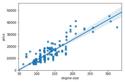
We can also view the correlation matrix for these two variables as follows
df[["engine-size", "price"]].corr()
| engine-size | price | |
|---|---|---|
| engine-size | 1.000000 | 0.872335 |
| price | 0.872335 | 1.000000 |
From this we can see that engine size is a fairly good predictor of price
Negative Correlation
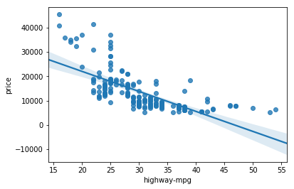
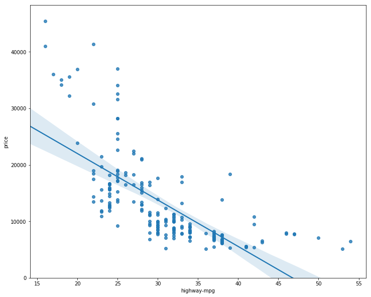
We can also look at the correation between highway mileage and price
sns.regplot(x="highway-mpg", y="price", data=df)
plt.show()
df[['highway-mpg', 'price']].corr()
| highway-mpg | price | |
|---|---|---|
| highway-mpg | 1.000000 | -0.704692 |
| price | -0.704692 | 1.000000 |
Where we can note a Negative Linear Relationship
Weak Correlation
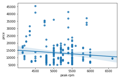
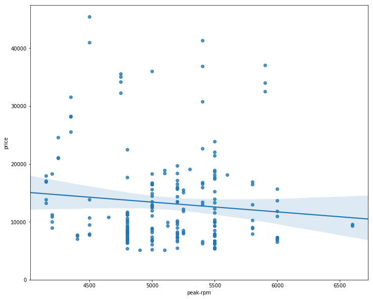
We can the compare Peak RPM and price
sns.regplot(x="peak-rpm", y="price", data=df)
plt.show()
df[['peak-rpm','price']].corr()
| peak-rpm | price | |
|---|---|---|
| peak-rpm | 1.000000 | -0.101616 |
| price | -0.101616 | 1.000000 |
Where we can see a weak linear relationship
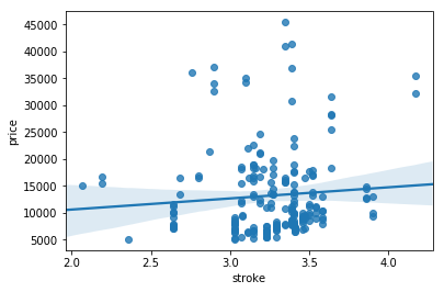
We can also observe the relationships between stroke and price
sns.regplot(x="stroke", y="price", data=df)
plt.show()
df[["stroke","price"]].corr()
| stroke | price | |
|---|---|---|
| stroke | 1.000000 | 0.082269 |
| price | 0.082269 | 1.000000 |
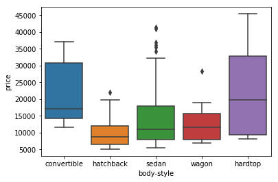
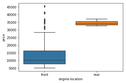
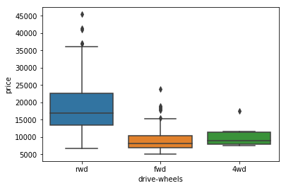
Next we can look at boxplots of our different categorical values in order to look at their distribution
sns.boxplot(x="body-style", y="price", data=df)
plt.show()
/opt/conda/envs/DSX-Python35/lib/python3.5/site-packages/seaborn/categorical.py:462: FutureWarning: remove_na is deprecated and is a private function. Do not use.
  box_data = remove_na(group_data)
sns.boxplot(x="engine-location", y="price", data=df)
plt.show()
/opt/conda/envs/DSX-Python35/lib/python3.5/site-packages/seaborn/categorical.py:462: FutureWarning: remove_na is deprecated and is a private function. Do not use.
  box_data = remove_na(group_data)
sns.boxplot(x="drive-wheels", y="price", data=df)
plt.show()
/opt/conda/envs/DSX-Python35/lib/python3.5/site-packages/seaborn/categorical.py:462: FutureWarning: remove_na is deprecated and is a private function. Do not use.
  box_data = remove_na(group_data)
Descriptive Statistics
Next we can find some descriptive statistics about our data by the following
df.describe()
| symboling | normalized-losses | wheel-base | length | width | height | curb-weight | engine-size | bore | stroke | ... | peak-rpm | city-mpg | highway-mpg | price | city-L/100km | highway-L/100km | fuel-type-diesel | fuel-type-gas | aspiration-std | aspiration-turbo | |
|---|---|---|---|---|---|---|---|---|---|---|---|---|---|---|---|---|---|---|---|---|---|
| count | 201.000000 | 201.00000 | 201.000000 | 201.000000 | 201.000000 | 201.000000 | 201.000000 | 201.000000 | 201.000000 | 201.000000 | ... | 201.000000 | 201.000000 | 201.000000 | 201.000000 | 201.000000 | 201.000000 | 201.000000 | 201.000000 | 201.000000 | 201.000000 |
| mean | 0.840796 | 122.00000 | 98.797015 | 0.837102 | 0.915126 | 0.899108 | 2555.666667 | 126.875622 | 3.330692 | 3.256874 | ... | 5117.665368 | 25.179104 | 30.686567 | 13207.129353 | 9.944145 | 8.044957 | 0.099502 | 0.900498 | 0.820896 | 0.179104 |
| std | 1.254802 | 31.99625 | 6.066366 | 0.059213 | 0.029187 | 0.040933 | 517.296727 | 41.546834 | 0.268072 | 0.316048 | ... | 478.113805 | 6.423220 | 6.815150 | 7947.066342 | 2.534599 | 1.840739 | 0.300083 | 0.300083 | 0.384397 | 0.384397 |
| min | -2.000000 | 65.00000 | 86.600000 | 0.678039 | 0.837500 | 0.799331 | 1488.000000 | 61.000000 | 2.540000 | 2.070000 | ... | 4150.000000 | 13.000000 | 16.000000 | 5118.000000 | 4.795918 | 4.351852 | 0.000000 | 0.000000 | 0.000000 | 0.000000 |
| 25% | 0.000000 | 101.00000 | 94.500000 | 0.801538 | 0.890278 | 0.869565 | 2169.000000 | 98.000000 | 3.150000 | 3.110000 | ... | 4800.000000 | 19.000000 | 25.000000 | 7775.000000 | 7.833333 | 6.911765 | 0.000000 | 1.000000 | 1.000000 | 0.000000 |
| 50% | 1.000000 | 122.00000 | 97.000000 | 0.832292 | 0.909722 | 0.904682 | 2414.000000 | 120.000000 | 3.310000 | 3.290000 | ... | 5125.369458 | 24.000000 | 30.000000 | 10295.000000 | 9.791667 | 7.833333 | 0.000000 | 1.000000 | 1.000000 | 0.000000 |
| 75% | 2.000000 | 137.00000 | 102.400000 | 0.881788 | 0.925000 | 0.928094 | 2926.000000 | 141.000000 | 3.580000 | 3.410000 | ... | 5500.000000 | 30.000000 | 34.000000 | 16500.000000 | 12.368421 | 9.400000 | 0.000000 | 1.000000 | 1.000000 | 0.000000 |
| max | 3.000000 | 256.00000 | 120.900000 | 1.000000 | 1.000000 | 1.000000 | 4066.000000 | 326.000000 | 3.940000 | 4.170000 | ... | 6600.000000 | 49.000000 | 54.000000 | 45400.000000 | 18.076923 | 14.687500 | 1.000000 | 1.000000 | 1.000000 | 1.000000 |
8 rows × 22 columns
df.describe(include=['object'])
| make | num-of-doors | body-style | drive-wheels | engine-location | engine-type | num-of-cylinders | fuel-system | |
|---|---|---|---|---|---|---|---|---|
| count | 201 | 201 | 201 | 201 | 201 | 201 | 201 | 201 |
| unique | 22 | 2 | 5 | 3 | 2 | 6 | 7 | 8 |
| top | toyota | four | sedan | fwd | front | ohc | four | mpfi |
| freq | 32 | 115 | 94 | 118 | 198 | 145 | 157 | 92 |
Value Counts
We can get an indication as to the frequencies of our categorical values with the following
# drive-wheel counts as a variable
drive_wheels_counts = df['drive-wheels'].value_counts().to_frame()
drive_wheels_counts.rename(columns={'drive-wheels': 'value_counts'}, inplace=True)
drive_wheels_counts
drive_wheels_counts.index.name = 'drive-wheels'
drive_wheels_counts
| value_counts | |
|---|---|
| drive-wheels | |
| fwd | 118 |
| rwd | 75 |
| 4wd | 8 |
# engine-location as variable
engine_loc_counts = df['engine-location'].value_counts().to_frame()
engine_loc_counts.rename(columns={'engine-location': 'value_counts'}, inplace=True)
engine_loc_counts.index.name = 'engine-location'
engine_loc_counts.head(10)
| value_counts | |
|---|---|
| engine-location | |
| front | 198 |
| rear | 3 |
Grouping Data
It can be helpful to group data in order to see if there is a correlation between a certain categorical data and some other variable
We can get an array of all uniques 'drive-wheel' categories with
df['drive-wheels'].unique()
array(['rwd', 'fwd', '4wd'], dtype=object)
In Pandas we can use df.groupby()to do this as such
df_wheels = df[['drive-wheels','body-style','price']]
df_wheels = df_wheels.groupby(['drive-wheels'],as_index= False).mean()
df_wheels
| drive-wheels | price | |
|---|---|---|
| 0 | 4wd | 10241.000000 |
| 1 | fwd | 9244.779661 |
| 2 | rwd | 19757.613333 |
Next we can look at the wheels compared to the body style
df_external = df[['drive-wheels', 'body-style', 'price']]
df_group = df_external = df_external.groupby(['drive-wheels','body-style'],
                                            as_index=False).mean().round()
df_group
| drive-wheels | body-style | price | |
|---|---|---|---|
| 0 | 4wd | hatchback | 7603.0 |
| 1 | 4wd | sedan | 12647.0 |
| 2 | 4wd | wagon | 9096.0 |
| 3 | fwd | convertible | 11595.0 |
| 4 | fwd | hardtop | 8249.0 |
| 5 | fwd | hatchback | 8396.0 |
| 6 | fwd | sedan | 9812.0 |
| 7 | fwd | wagon | 9997.0 |
| 8 | rwd | convertible | 23950.0 |
| 9 | rwd | hardtop | 24203.0 |
| 10 | rwd | hatchback | 14338.0 |
| 11 | rwd | sedan | 21712.0 |
| 12 | rwd | wagon | 16994.0 |
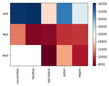
We can view this data a bit more conviniently as a pivot table, we can do this with df.pivot() so as to display the data as below
grouped_pivot = df_group.pivot(index='drive-wheels',columns='body-style')
grouped_pivot
| price | |||||
|---|---|---|---|---|---|
| body-style | convertible | hardtop | hatchback | sedan | wagon |
| drive-wheels | |||||
| 4wd | NaN | NaN | 7603.0 | 12647.0 | 9096.0 |
| fwd | 11595.0 | 8249.0 | 8396.0 | 9812.0 | 9997.0 |
| rwd | 23950.0 | 24203.0 | 14338.0 | 21712.0 | 16994.0 |
Next we can use a heatmap to visualize the above relationship, the heatmap plots the target variable as the colour with respect to the drive-wheels and body-style variables
#use the grouped results
fig, ax = plt.subplots()
im=ax.pcolor(grouped_pivot, cmap='RdBu')

#label names
row_labels=grouped_pivot.columns.levels[1]
col_labels=grouped_pivot.index

#move ticks and labels to the center
ax.set_xticks(np.arange(grouped_pivot.shape[1])+0.5, minor=False)
ax.set_yticks(np.arange(grouped_pivot.shape[0])+0.5, minor=False)

#insert labels
ax.set_xticklabels(row_labels, minor=False)
ax.set_yticklabels(col_labels, minor=False)

#rotate label if too long
plt.xticks(rotation=90)

fig.colorbar(im)
plt.show()
Analysis of Variance (ANOVA)
If we want to analyze a categorical variable and see the correlation between different categories
- Statistical comparison of groups
ANOVA is a statistical test that hels find the correlation between different groups of a categorical variable, the ANOVA returns two values
- F-Test score is the variation between sample group means divided by variation within the sample group
- P-Value is a measure of confidence and show if the obtained result is statistically significant
Drive Wheels
grouped_test2=df[['drive-wheels','price']].groupby(['drive-wheels'])
grouped_test2.head(2)
| drive-wheels | price | |
|---|---|---|
| 0 | rwd | 13495.0 |
| 1 | rwd | 16500.0 |
| 3 | fwd | 13950.0 |
| 4 | 4wd | 17450.0 |
| 5 | fwd | 15250.0 |
| 136 | 4wd | 7603.0 |
grouped_test2.get_group('4wd')['price']
4      17450.0
136     7603.0
140     9233.0
141    11259.0
144     8013.0
145    11694.0
150     7898.0
151     8778.0
Name: price, dtype: float64
To obtain the ANOVA values, we use the stats.f_oneway function from scipy for the correlation between drive wheels and price
Drive Wheels and Price
# ANOVA
f_val, p_val = stats.f_oneway(grouped_test2.get_group('fwd')['price'], grouped_test2.get_group('rwd')['price'], grouped_test2.get_group('4wd')['price'])

print( "ANOVA results: F=", f_val, ", P =", p_val)
ANOVA results: F= 67.9540650078 , P = 3.39454435772e-23
This shows a large F and small P, meaning that there is a strong corelation between the three drive types and the price, however does this apply for each individual comparison of drive type?
FWD and RWD
f_val, p_val = stats.f_oneway(grouped_test2.get_group('fwd')['price'], grouped_test2.get_group('rwd')['price'])

print( "ANOVA results: F=", f_val, ", P =", p_val )
ANOVA results: F= 130.553316096 , P = 2.23553063557e-23
4WD and RWD
f_val, p_val = stats.f_oneway(grouped_test2.get_group('4wd')['price'], grouped_test2.get_group('rwd')['price'])

print( "ANOVA results: F=", f_val, ", P =", p_val)
ANOVA results: F= 8.58068136892 , P = 0.00441149221123
4WD and FWD
f_val, p_val = stats.f_oneway(grouped_test2.get_group('4wd')['price'], grouped_test2.get_group('fwd')['price'])

print("ANOVA results: F=", f_val, ", P =", p_val)
ANOVA results: F= 0.665465750252 , P = 0.416201166978
Model Development
A model can be thought of as a mathematical equation used to predict a value given a specfic input
More relevant data will allow us to more accurately predict an outcome
Linear Regression
Simple Linear Regression
SLR helps us to identify a relationship between two independant variables in the form of
We make use of training datapoints to help us find the and values
Our measured datapoints will have some noise, causing our data to be differerntiated from the model
We make use of our training data to fit a model to our data, we then use the model to make predictions. We denote our predicted values as an estimate with
If the linear model is correct, we can assume that the offsets are noise, otherwise it may be other factors that we have not taken into consideration
We can create a linear regression model by importing it from sklearn and creating a new LinearRegression object as follows
from sklearn.linear_model import LinearRegression

lm = LinearRegression()
Then we define the predictor and target variables and use lm.fit() to find the parameters and
X = df[['predictor']]
Y = df[['target']]

lm.fit(X,Y)
We can then obtain a prediction using `lm.predict()'
yhat = lm.predict(X)
The intercept and slope are attributes of the LinearRegression object and can be found with lm.intercept_ and lm.coef_ respectively
We can train an SLR model for our data as follows
df.head()
| symboling | normalized-losses | make | num-of-doors | body-style | drive-wheels | engine-location | wheel-base | length | width | ... | city-mpg | highway-mpg | price | city-L/100km | highway-L/100km | horsepower-binned | fuel-type-diesel | fuel-type-gas | aspiration-std | aspiration-turbo | |
|---|---|---|---|---|---|---|---|---|---|---|---|---|---|---|---|---|---|---|---|---|---|
| 0 | 3 | 122 | alfa-romero | two | convertible | rwd | front | 88.6 | 0.811148 | 0.890278 | ... | 21 | 27 | 13495.0 | 11.190476 | 8.703704 | Medium | 0 | 1 | 1 | 0 |
| 1 | 3 | 122 | alfa-romero | two | convertible | rwd | front | 88.6 | 0.811148 | 0.890278 | ... | 21 | 27 | 16500.0 | 11.190476 | 8.703704 | Medium | 0 | 1 | 1 | 0 |
| 2 | 1 | 122 | alfa-romero | two | hatchback | rwd | front | 94.5 | 0.822681 | 0.909722 | ... | 19 | 26 | 16500.0 | 12.368421 | 9.038462 | Medium | 0 | 1 | 1 | 0 |
| 3 | 2 | 164 | audi | four | sedan | fwd | front | 99.8 | 0.848630 | 0.919444 | ... | 24 | 30 | 13950.0 | 9.791667 | 7.833333 | Medium | 0 | 1 | 1 | 0 |
| 4 | 2 | 164 | audi | four | sedan | 4wd | front | 99.4 | 0.848630 | 0.922222 | ... | 18 | 22 | 17450.0 | 13.055556 | 10.681818 | Medium | 0 | 1 | 1 | 0 |
5 rows × 31 columns
from sklearn.linear_model import LinearRegression
X = df[['highway-mpg']]
Y = df['price']
lm = LinearRegression()
lm.fit(X,Y)
LinearRegression(copy_X=True, fit_intercept=True, n_jobs=1, normalize=False)
Yhat=lm.predict(X)
Yhat[0:5]
array([ 16236.50464347,  16236.50464347,  17058.23802179,  13771.3045085 ,
        20345.17153508])
lm_eq = 'yhat = ' + str(lm.intercept_) + ' + ' + str(lm.coef_[0]) + 'x'
print(lm_eq)
yhat = 38423.3058582 + -821.733378322x
Multiple Linear Regression
MLR is used to explain the relationship between 1 continuous target and 2 or more predictors
The model will then be defined by the function
The resulting equation represents a surface in dimensional space that will define given each component of
We can train this model just as before as follows
X = df[['predictor1','predictor2','predictor3',...,'predictorN']]
Y = df[['target']]

lm.fit(X,Y)
And then predict as before with
yhat = lm.predict(X)
Where X is in the form of the training data
The intercept and coefficiencts of the model can once again be found with lm.intercept_ and lm.coef_ respectively
We can develop a MLR model as follows
Z = df[['horsepower', 'curb-weight', 'engine-size', 'highway-mpg']]
lm.fit(Z, df['price'])
print('intercept: ' + str(lm.intercept_), '\ncoefficients: ' + str(lm.coef_))
intercept: -15806.6246263
coefficients: [ 53.49574423   4.70770099  81.53026382  36.05748882]
Model Evaluation using Visualization
Regression Plot
Regression plots gives us a good estimate of:
- The relationship between two variables
- The strength of correlation
- The direction of the relationship
A regression plot is a combination of a scatter plot, and a linear regression line
We create a regression plot using the sns.regplot() function in seaborn
import seaborn as sns

sns.regplot(x='predictor', y='target', data=df)
plt.ylim(0,)
plt.show()
Single Linear Regression
We can visualize SLR as follows
width = 12
height = 10
plt.figure(figsize=(width, height))
sns.regplot(x="highway-mpg", y="price", data=df)
plt.ylim(0,)
plt.show()
plt.figure(figsize=(width, height))
sns.regplot(x="peak-rpm", y="price", data=df)
plt.ylim(0,)
(0, 47422.919330307624)
Residual Plot
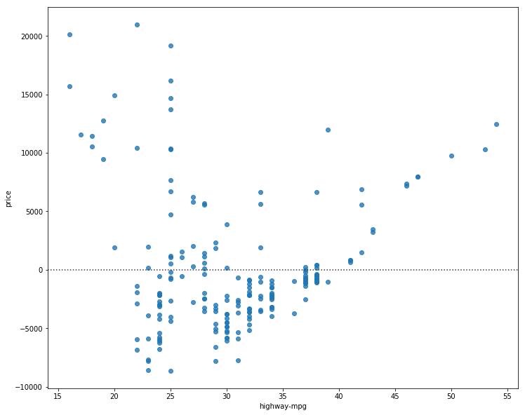
A Residual plot represents the error between the actual and predicted value, the results should have 0 mean if the linear assumption is applicable
If the residual plot is not equally distributed around the mean of 0 throughout, we know that the linear model is not correct for the data we have
We can create a residual plot as with sns.residplot()
sns.residplot(df['predictor'], df['target'])
width = 12
height = 10
plt.figure(figsize=(width, height))
sns.residplot(df['highway-mpg'], df['price'])
plt.show()
Distribution Plot
We use this to look at the distribution of the actual vs predicted values for our model
A distribution plot can be made with sns.distplot()
ax1 = sns.distplot(df['target'], hist=False, label='Actual Value')
sns.distplot(yhat, hist=False, label='Fitted Values', ax=ax1)
plt.show()
Multiple Linear Regression
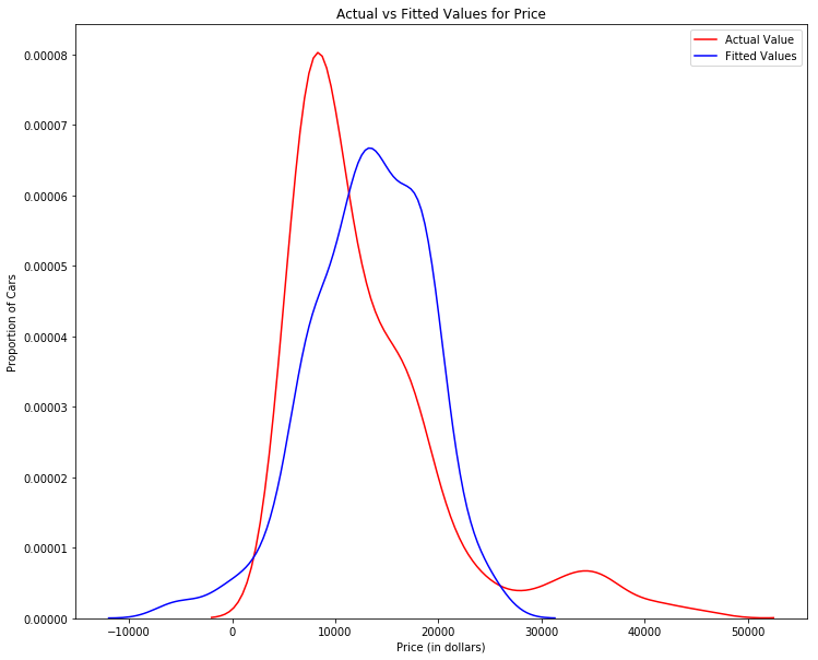
Using A Distribution Plot is more valuable when looking at MLR model performance
Y_hat = lm.predict(Z)
plt.figure(figsize=(width, height))


ax1 = sns.distplot(df['price'], hist=False, color="r", label="Actual Value")
sns.distplot(Yhat, hist=False, color="b", label="Fitted Values" , ax=ax1)


plt.title('Actual vs Fitted Values for Price')
plt.xlabel('Price (in dollars)')
plt.ylabel('Proportion of Cars')

plt.show()
plt.close()
Polynomial Regression and Pipelines
Polynomial Regression is a form of regression used to describe curvilinear relationships in which our predictor variable is not linear
- Quadratic
- Cubic
- Higher Order
Picking the correct order can make our model more accurate
We can fit a polynomial to our data using np.polyfit(), and can print out the resulting model with np.polydl()
For an order polynomial we can create and view a model as follows
model = np.polyfit(X,Y,n)
print(np.polydl(f))
Visualization
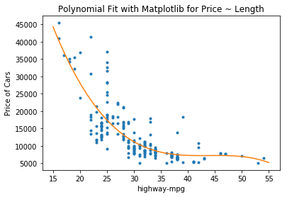
Visualizing Polynomial regression plots is a bit more work but can be done with the function below
def PlotPolly(model,independent_variable,dependent_variabble, Name):
    x_new = np.linspace(15, 55, 100)
    y_new = model(x_new)

    plt.plot(independent_variable,dependent_variabble,'.', x_new, y_new, '-')
    plt.title('Polynomial Fit with Matplotlib for Price ~ Length')
    ax = plt.gca()
    fig = plt.gcf()
    plt.xlabel(Name)
    plt.ylabel('Price of Cars')

    plt.show()
    plt.close()
Next we can do the polynomial fit for our data
x = df['highway-mpg']
y = df['price']

f = np.polyfit(x, y, 3)
p = np.poly1d(f)
print(p)
        3         2
-1.557 x + 204.8 x - 8965 x + 1.379e+05
PlotPolly(p,x,y, 'highway-mpg')
Multi Dimension Polynomial Regression
Polynomial regression can also be done in multiple dimensions, for example a second order approximation would look like the following
If we want to do multi dimentional polynomial fits, we will need to use PolynomialFeatures from sklearn.preprocessing to preprocess our features as follows
X = df[['predictor1','predictor2','predictor3',...,'predictorN']]
Y = df[['target']]

pr = PolynomialFeatures(degree=2)
x_poly = pr.fit_transform(X, include_bias=False)
from sklearn.preprocessing import PolynomialFeatures
pr = PolynomialFeatures(degree=2)
pr
PolynomialFeatures(degree=2, include_bias=True, interaction_only=False)
Z_pr = pr.fit_transform(Z)
Before the transformation we have 4 features
Z.shape
(201, 4)
After the transformation we have 15 features
Z_pr.shape
(201, 15)
Pre-Processing
sklearn has some preprocessing functionality such as
Normalization
We can train a scaler and normalize our data based on that as follows
from sklearn.preprocessing import StandardScaler

scale = StandardScaler()
scale.fit(X[['feature1','feature2',..., 'featureN']])

X_scaled = scale.transform(X[['feature1','feature2',..., 'featureN']])
There are other normalization functions available with which we can preprocess our data
Pipelines
There are many steps to getting a prediction, such as Normalization, Polynomial Transformation, and training a Linear Regression Model
We can use a Pipeline library to help simplify the process
First we import all the libraries we will need as well as the pipeline library
from sklearn.preprocessing import PolynomialFeatures
from sklearn.linear_model import LinearRegression
from sklearn.preprocessing import StandardScaler

from sklearn.pipeline import Pipeline
Then we construct our pipeline using a list of tuples defined as ('name of estimator model', ModelConstructor()) and create our pipeline object
input = [('scale', StandardScaler()),
         ('polynomial', PolynomialFeatures(degree=n),
         ...,
         ('mode', LinearRegression()]
pipe = Pipeline(Input)
We can then create our pipeline object on the data by using the pipe.train function
pipe.train(X[['feature1','feature2',..., 'featureN']], Y)
yhat = pipe.predict(X[['feature1','feature2',..., 'featureN']])
The above method will normalize the data, then perform a polynomial transform and output a prediction
from sklearn.pipeline import Pipeline
from sklearn.preprocessing import StandardScaler
Input=[('scale',StandardScaler()),
       ('polynomial', PolynomialFeatures(include_bias=False)),
       ('model',LinearRegression())]
pipe=Pipeline(Input)
pipe
Pipeline(memory=None,
     steps=[('scale', StandardScaler(copy=True, with_mean=True, with_std=True)), ('polynomial', PolynomialFeatures(degree=2, include_bias=False, interaction_only=False)), ('model', LinearRegression(copy_X=True, fit_intercept=True, n_jobs=1, normalize=False))])
pipe.fit(Z,y)
Pipeline(memory=None,
     steps=[('scale', StandardScaler(copy=True, with_mean=True, with_std=True)), ('polynomial', PolynomialFeatures(degree=2, include_bias=False, interaction_only=False)), ('model', LinearRegression(copy_X=True, fit_intercept=True, n_jobs=1, normalize=False))])
ypipe=pipe.predict(Z)
ypipe[0:4]
array([ 13102.74784201, 13102.74784201, 18225.54572197, 10390.29636555])
In-Sample Evaluation
Two important measures that determine how well a model fits a speficic dataset are
- Mean Squared Error (MSE)
- R-Squared ()
Mean Squared Error
We simply find the difference between the average square error of our prediction when compared to our data
To get the MSE in Python we can do the following
from sklearn.metrics import mean_squared_error

mean_squared_error(X['target'],Y_predicted_sample)
R-Squared
is the coefficient of determination
- Measure of how close the data is to the fitted regression line
- The percentage of variation in Y that is explained by the model
- Like comparing our model to the mean of the data in approximating the data
is usually between 0 and 1
We can get the value with lm.score()
A negative can be a sign of overfitting
In-Sample Evaluation of Models
We can evaluate our models with the following
#highway_mpg_fit
lm.fit(X, Y)
# Find the R^2
lm.score(X, Y)
0.49659118843391747
Yhat = lm.predict(X)
Yhat[0:4]
array([ 16236.50464347, 16236.50464347, 17058.23802179, 13771.3045085 ])
from sklearn.metrics import mean_squared_error
#mean_squared_error(Y_true, Y_predict)
mean_squared_error(df['price'], Yhat)
31635042.944639895
# fit the model
lm.fit(Z, df['price'])
# Find the R^2
lm.score(Z, df['price'])
0.80935628065774567
Y_predict_multifit = lm.predict(Z)
mean_squared_error(df['price'], Y_predict_multifit)
11980366.87072649
Now we can check what the value for our model is
from sklearn.metrics import r2_score
r_squared = r2_score(y, p(x))
r_squared
0.67419466639065173
mean_squared_error(df['price'], p(x))
20474146.426361222
Prediction and Decision Making
We should use visualization, numerical evaluation, and model comparison in order to see if the model values makes sense
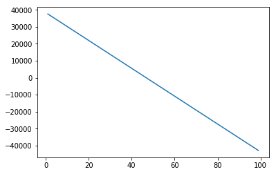
To compare our model to the data we can simply plot the output of our model over the range of our data
new_input=np.arange(1,100,1).reshape(-1,1)
lm.fit(X, Y)
LinearRegression(copy_X=True, fit_intercept=True, n_jobs=1, normalize=False)
yhat=lm.predict(new_input)
yhat[0:5]
array([ 37601.57247984,  36779.83910151,  35958.10572319,  35136.37234487,
        34314.63896655])
plt.plot(new_input,yhat)
plt.show()
Conclusion
From the results above (yes, they're a mess but it's all pretty much just from the CC Lab file) we can note the and MSE values are as follows
Simple Linear Regression: Using Highway-mpg as a Predictor Variable of Price.
- R-squared: 0.49659118843391759
- MSE: 3.16 x10^7
Multiple Linear Regression: Using Horsepower, Curb-weight, Engine-size, and Highway-mpg as Predictor Variables of Price.
- R-squared: 0.80896354913783497
- MSE: 1.2 x10^7
Polynomial Fit: Using Highway-mpg as a Predictor Variable of Price.
- R-squared: 0.6741946663906514
- MSE: 2.05 x 10^7
SLR vs MLR
Usually having more variables helps the prediction, however if you do not have enough data you can run into trouble or many of the variables may just be noise and not be very useful
The MSE for MLR is Smaller than for SLR, and the for MLR is higher as well, MSE and both seem to indicate that MLR is a better fit than SLR
SLR vs Polynomial
The MSE for the Polynomial Fit is less than for the SLR and the is higher meaning that the Polynomial Fit is a better predictor based on 'highway-mpg' than the SLR
MLR vs Polynomial
The MSE for the MLR is smaller than for the Polynomial Fit, and the MLR also has a higher therefore the MLR is as better fit than the Polynomial in this case
Overall
The MLR has the lowest and the highest MSE, meaning that it is the best fit of the three models that have been evaluate
Model Evaluation
Model Evaluation tells us how our model works in the real wold. In-Sample evaluation does not give us an indication as to how our model performs under real lifr circumstances
Training and Test Sets
We typically split our data into a training and testing set and use to build and evaluate our model respectively
- Split into
- 70% Training
- 30% Testing
- Build and Train with Training Set
- Use Testing Set to evaluate model performance
sklearn gives us a function to split out data into a train and test set
from sklearn.model_selection import train_test_split

X_train, X_test, Y_train, Y_test = train_test_split(x_data,y_data,test_size=0.3,random_state=0)
Generalization Performance
Generalization Error is a measure of how well our data does at predicting previously unseen data
The error we obtain using our testing data is an approximation of this error
Cross Validation
Cross validation involves us splitting the data into folds and using a fold for testing and the remainder for training, and we make use of each combination of training, and evalution
We can use cross_val_score() to evaluate our out-of-sample evaluation
from sklearn.model_selection import cross_val_score
scores = cross_val_score(lr,X,Y,cv=n)
Where X is our predictor matrix, Y is our target, and n is our number of folds
If we want to use get the actual predicted values from our model we can do the following
from sklearn.model_selection import cross_val_predict
yhat = cross_val_predict(lr,X,Y,cv=n)
Overfitting, Underfitting, and Model Selection
The goal of model selection is to try to select the best function to fit our model, if our model is too simple we will have model that does not appropriately fit our data, whereas if we have a model that is too complex, it wil perfectly fit our testing data but will not be good at approximating new data
We need to be sure to fit the data, not the noise
It is also possible that the data we are trying to approximate cannot be fitted by polynomial at all, for example in the case of cyclic data
We can make use of the following code to look at the effect of order on our error for a model
rsq_test = []
order = [1,2,3,4]

for n in order:
    pr = PolynomialFeatures(degree=n)
    x_train_pr = pr.fit_transform(x_train[['feature']]
    x_test_pr = pr.fit_transform(x_test[['feature']]
    lm.fit(x_train_pr, y_train)
    rsq_test.append(lr.score(x_test_pr, y_test))
Ridge Regression
Ridge Regression prevents overfitting
Ridge regression controls the higher order parameters in our model by using a factor , increasing our value will help us avoid overfitting until, however increasing it too far can lead to us underfitting the data
To use ridge regression we can do the following
from sklearn.linear_model import Ridge

ridge_model = Ridge(alpha=0.1)
ridge_model.fit(X,Y)
yhat=RidgeModel.predict(X)
We will usually start off with a small value of such as 0.0001 and increase our value in orders of magnitude
Furthermore we can use Cross Validation to identify an optimal
Grid Search
Grid Search allows us to scan through multiple free parameters
Parameters such as are not part of the training or fitting process. These parameters are called Hyperparameters
sklearn has a means of automatically iterating over these parameters called Grid Search
This allows us to use different hyperparameters to train our model, and select the model that provides the lowest MSE
The values of a grid search are simply a list whcih contains a dictionary for the parameters we want to modify
params = [{'param name':[value1, value2, value3, ...]}]
We can use Grid Search as follows
from sklearn.linear_model import Ridge
from sklearn.model_selection import GridSearchCV

params = [{'alpha':[0.0001, 0.01, 1, 10, 100]}, {'normalize':[True,False]}]

rr = Ridge()

grid = GridSearchCV(rr, params, cv=4)
grid.fit(X_train[['feature1','feature2',...], Y_train)

grid.best_estimator_

scores = grid.cv_results_
The scores dictionary will store the results for each hyperparameter combination given our inputs
Conclusion
For more specific examples of the different setions look at the appropriate Lab